Comparing meanings: a worked example

library(actdata)
library(dplyr)
#> 
#> Attaching package: 'dplyr'
#> The following objects are masked from 'package:stats':
#> 
#>     filter, lag
#> The following objects are masked from 'package:base':
#> 
#>     intersect, setdiff, setequal, union
library(tidyr)
library(ggplot2)

The Tidyverse makes it easy to create new combinations or subsets of ACT dictionaries in a way that is completely replicable, and to visualize quantities of interest over time and/or across countries. An example of how these data sets can be used along with dplyr, tidyr, and ggplot is presented here.

Say we are interested in comparing changes in evaluation ratings for terms over time in whatever countries possible. The table on the dictionaries help page shows that the three countries in which multiple dictionaries have been collected are the U.S., Canada, and Germany. Let’s choose three U.S. dictionaries (nc1978, texas1998, and usfullsurveyor2015), two Canadian dictionaries (ontario1980 and ontario2001), and two German dictionaries (germany1989 and germany2007). Now we need to find the terms that are in all seven dictionaries. The term table is useful to quickly get a first look at this.

datasets <- c("nc1978", "texas1998", "usfullsurveyor2015", "ontario1980", "ontario2001", "germany1989", "germany2007")

term_table_short <- term_table %>% 
  # we only need the columns for our chosen dictionaries
  select(term, component, all_of(datasets)) %>% 
  # filter to those terms present in all chosen dictionaries
  filter(if_all(datasets, ~ . == 1))
#> Warning: Using an external vector in selections was deprecated in tidyselect 1.1.0.
#> ℹ Please use `all_of()` or `any_of()` instead.
#>   # Was:
#>   data %>% select(datasets)
#> 
#>   # Now:
#>   data %>% select(all_of(datasets))
#> 
#> See <https://tidyselect.r-lib.org/reference/faq-external-vector.html>.
#> This warning is displayed once every 8 hours.
#> Call `lifecycle::last_lifecycle_warnings()` to see where this warning was
#> generated.

head(term_table_short)
#> # A tibble: 6 × 9
#>   term     component nc1978 texas1998 usfullsurveyor2015 ontario1980 ontario2001
#>   <chr>    <chr>      <dbl>     <dbl>              <dbl>       <dbl>       <dbl>
#> 1 champion identity       1         1                  1           1           1
#> 2 child    identity       1         1                  1           1           1
#> 3 hero     identity       1         1                  1           1           1
#> 4 idiot    identity       1         1                  1           1           1
#> 5 judge    identity       1         1                  1           1           1
#> 6 librari… identity       1         1                  1           1           1
#> # ℹ 2 more variables: germany1989 <dbl>, germany2007 <dbl>

We now have a list of the 225 identities included in all seven dictionaries. Let’s get the mean EPA values for these terms.

# trim the term table further to get rid of the dataset key columns
term_table_forfilter <- term_table_short %>% 
  select(term, component)

# Now, merge this list with the EPA summary dataset to get epa values for the countries and years we are interested in.
# First, subset the epa summary dataframe to the dictionaries we want, to only include means, and to only include gender averaged values.
term_subset <- epa_subset(dataset = datasets, stat = "mean", group = "all") %>% 
  # then right join with the term list we built before to subset to only the terms we are interested in. 
  right_join(term_table_forfilter, by = c("term", "component")) %>% 
  arrange(term)

term_subset[1:20,]
#> # A tibble: 20 × 10
#>    term     component dataset context year  group instcodes      E      P      A
#>    <chr>    <chr>     <chr>   <chr>   <chr> <chr> <chr>      <dbl>  <dbl>  <dbl>
#>  1 academic identity  german… Germany 1989  all   11 00001…  0.81   0.54  -0.765
#>  2 academic identity  german… Germany 2007  all   11 00001…  1.60   1.25  -0.125
#>  3 academic identity  nc1978  US      1978  all   11 00001…  0.975  0.735 -0.5  
#>  4 academic identity  ontari… Canada  1980  all   11 00001…  1.38   1.04  -0.42 
#>  5 academic identity  ontari… Canada  2001  all   11 00001…  1.64   1.23   0.235
#>  6 academic identity  texas1… US      1998  all   11 00001…  1.83   1.69   0.37 
#>  7 academic identity  usfull… US      2015  all   11 00001…  2.34   2.26  -0.12 
#>  8 adopt    behavior  german… Germany 1989  all   10 00000…  1.8   -0.265 -0.485
#>  9 adopt    behavior  german… Germany 2007  all   10 00000…  2.24   1.77  -0.235
#> 10 adopt    behavior  nc1978  US      1978  all   10 00000…  1.92   1.56   0.035
#> 11 adopt    behavior  ontari… Canada  1980  all   10 00000…  2.41   1.04   0.33 
#> 12 adopt    behavior  ontari… Canada  2001  all   10 00000…  2.30   1.58   0.755
#> 13 adopt    behavior  texas1… US      1998  all   10 00000…  3.04   1.88   1.25 
#> 14 adopt    behavior  usfull… US      2015  all   10 00000…  3.12   2.88   0.15 
#> 15 adulter… identity  german… Germany 1989  all   10 00000… -1.6    0.445  0.745
#> 16 adulter… identity  german… Germany 2007  all   10 00000… -2.46   0.365  0.68 
#> 17 adulter… identity  nc1978  US      1978  all   10 00000… -1.80   0      0.855
#> 18 adulter… identity  ontari… Canada  1980  all   10 00000… -1.92   0.5    0.89 
#> 19 adulter… identity  ontari… Canada  2001  all   10 00000… -2.32  -0.09   0.31 
#> 20 adulter… identity  texas1… US      1998  all   10 00000… -2.77  -0.655  0.345

Now we have a dataframe that contains just the gender-averaged EPA values for the terms that the seven dictionaries share.

How are meanings changing overall? We can calculate meaning change summary statistics to get a better sense of this:

eval_change <- term_subset %>% 
  # get rid of the texas dataset here; just use the first and last US sets for a change calculation. Drop institution codes too, we won't use them here.
  filter(dataset != "texas1998") %>% 
  # first pivot longer so that there is one sentiment value per row
  pivot_longer(cols = c(E, P, A), names_to = "dimension", values_to = "rating") %>% 
  select(term, component, context, year, dimension, rating, -instcodes) %>%
  mutate(order = ifelse(year %in% c("2015", "2007", "2001"), "late", "early")) %>% 
  select(-year) %>% 
  # then pivot wider by time order
  pivot_wider(names_from = order, values_from = rating) %>% 
  # we get a warning here because there are a few duplicate terms. Clown, secretary, and waiter are all included more than once in the nc1978 data set. This is something to watch for; there are a handful of duplicates in other data sets as well. These are in the original raw data files and they have been left as is in this package. Here, I remove these terms. I also remove "no_emotion" here.
  filter(!(term %in% c("waiter", "clown", "secretary", "no_emotion"))) %>% 
  # now calculate change
  mutate(change = as.numeric(late) - as.numeric(early)) 
#> Warning: Values from `rating` are not uniquely identified; output will contain
#> list-cols.
#> • Use `values_fn = list` to suppress this warning.
#> • Use `values_fn = {summary_fun}` to summarise duplicates.
#> • Use the following dplyr code to identify duplicates.
#>   {data} |>
#>   dplyr::summarise(n = dplyr::n(), .by = c(term, component, context, dimension,
#>   order)) |>
#>   dplyr::filter(n > 1L)

summary(eval_change$change)
#>     Min.  1st Qu.   Median     Mean  3rd Qu.     Max. 
#> -3.09500 -0.30000  0.07000  0.08698  0.50000  2.68500

Mean and median change for all three countries are close to 0, suggesting broad stability in cultural meanings over time, but in all three datasets there are terms which change meaning substantially. Let’s find the terms that have undergone the biggest changes in meaning:

eval_change_substantial <- eval_change %>% 
  arrange(-abs(change))

head(eval_change_substantial)
#> # A tibble: 6 × 7
#>   term      component context dimension early     late      change
#>   <chr>     <chr>     <chr>   <chr>     <list>    <list>     <dbl>
#> 1 fool      identity  Germany A         <dbl [1]> <dbl [1]>  -3.10
#> 2 cajole    behavior  Germany A         <dbl [1]> <dbl [1]>  -2.7 
#> 3 cajole    behavior  Germany E         <dbl [1]> <dbl [1]>   2.68
#> 4 harm      behavior  Germany P         <dbl [1]> <dbl [1]>  -2.59
#> 5 doll      identity  US      A         <dbl [1]> <dbl [1]>  -2.51
#> 6 miserable modifier  Germany P         <dbl [1]> <dbl [1]>  -2.26

This data format is amenable to plotting with ggplot. Let’s look at a few of the terms which have seen substantial meaning change.

change_terms <- c("lesbian", "junkie", "depressed")

# I'm returning to the subset data frame here
terms_toplot <- term_subset %>% 
  filter(term %in% change_terms) %>% 
  rename(Evaluation = E, 
         Potency = P,
         Activity = A) %>% 
  pivot_longer(cols = c(Evaluation, Potency, Activity), names_to = "dimension", values_to = "rating") %>% 
  mutate(dimension = factor(dimension, levels = c("Evaluation", "Potency", "Activity")))

ggplot(terms_toplot, aes(x = as.numeric(year), y = rating, shape = context, color = term)) +
  geom_point(size = 2.5) +
  geom_line(alpha = .5) + 
  facet_wrap("dimension") + 
  labs(x = "Year",
       y = "Mean sentiment rating")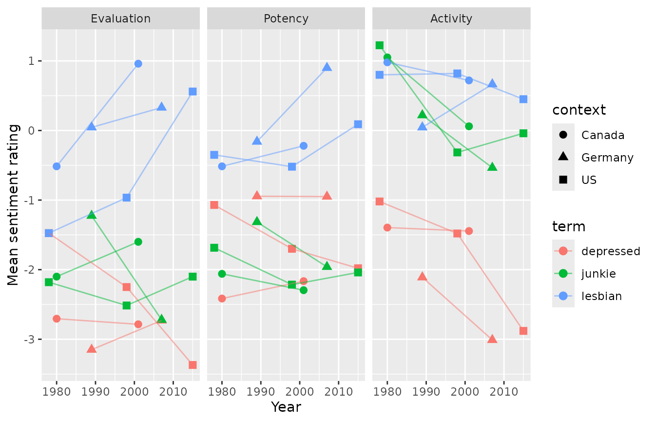

This shows that “lesbian” rose on the evaluation and power dimensions in all three countries and “junkie” fell on the activity dimension in all three countries. The trajectory of “depressed” was more place-dependent: it fell on all three dimensions in the US, stayed stable on evaluation and potency in Canada and Germany, and fell on activity in Germany. This type of analysis cannot show causation, of course, but it can be a useful start point for identifying and investigating terms that may have been affected by social movements or other shifts within and/or across countries. Similarly, this kind of analysis could be used to identify terms that vary across cultures, and, in cultures where multiple datasets have been collected, to investigate whether these differences have changed over time.